Jb Tak Fodega Nhi 🎯 Tb Tk Chodega Nhi 📚 (MAANG)

DPL37 Best Time to Buy and Sell Stock III

We are given an array Arr[] of length n. It represents the price of a stock on ‘n’ days. The following guidelines need to be followed:

We can buy and sell the stock any number of times.

In order to sell the stock, we need to first buy it on the same or any previous day.

We can’t buy a stock again after buying it once. In other words, we first buy a stock and then sell it. After selling we can buy and sell again. But we can’t sell before buying and can’t buy before selling any previously bought stock.

We can do at most 2 Transactions.

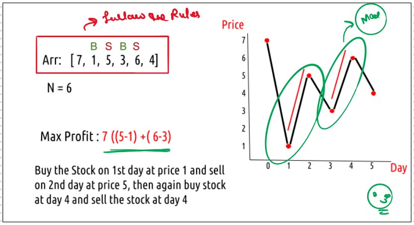
Find and return the maximum profit you can achieve.

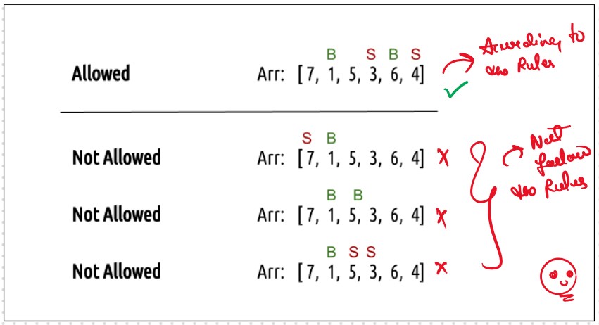
Only Few Updates in this Question As Compared to the Last, DPL36 Best Time to Buy and Sell Stock II

In Best Time to Buy and Sell Stock I: We Allow Just Only 1 Transactions

In Best Time to Buy and Sell Stock II: We Allow Infinite Transactions

In Best Time to Buy and Sell Stock III: We Allow Just Only 2 Transactions

In Best Time to Buy and Sell Stock III We Allow Just Only 2 Transactions Thsi Probelms Give a Reminder of the Knapsack Probelm that we all ready Done.
This Problem is the Application Varient of the Best Time to Buy and Sell Stock II, Just Only Modified the SOme Line of the Code

Add the Cap Variable in the Recursion, Memoization, tabluation and Space Optimization that Show the Limit of the 2

Just onlt Add the Cap Variable in the All the Code in Best Time to Buy and Sell Stock II that is the Only Single Change and Entire Logic and Code will be Same as we Done in Best Time to Buy and Sell Stock II

In Recursice Approch We Just Add the Cap Variable in the Recursion, Memoization, tabluation and Space Optimization that Show the Limit of the 2, and Modified Entire Solution on the Base of the Cap Variable

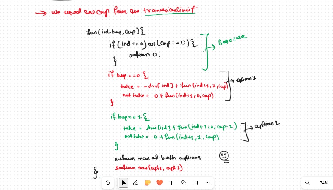
Now Here is the Question Why we:-

Option1: Not Change the Cap Value

Option2: We Changed the Cap Value

the Answe is Any transaction Whern Counted Completed, When we Buy and Sell the Stock And Gain Some Profit, So we Need to Change the Cap Value, and When we Not Buy and Sell the Stock, So we Not Need to Change the Cap Value. Buy Stock + Shell Stock = Count 1 Transaction

This is the Suffel Change Required in the Previous Code, and Everything will be Same Just use the Cap Variable and Modified all the Soltuions

Now Remaining Entire 👇 Process will Be Same As Like in DPL36

Every day, we will have two choices, either to do nothing and move to the next day or to buy/sell (based on the last transaction) and find out the profit. Therefore we need to generate all the choices in order to compare the profit. As we need to try out all the possible choices, we will use recursion.

Recursice Approch

Again here we follow the out Standerad Patter that we learned in the Dynamic Programming Introduction. How to Write Recursion

Steps to form the Recursive Solution
Step 1: Express the problem in terms of indexes.

We need to think in the terms of the number of days, therefore one variable will be the array index( say ind). Next, we need to respect the condition that we can’t buy a stock again, that is we need to first sell a stock, and then we can buy that again. Therefore we need a second variable ‘buy’ which tells us on a particular day whether we can buy or sell the stock. Next, we have a cap on the number of transactions that we can make. Here the initial cap is 2. We need to always keep in mind this constraint.

Step 2: Try out all possible choices at a given index.

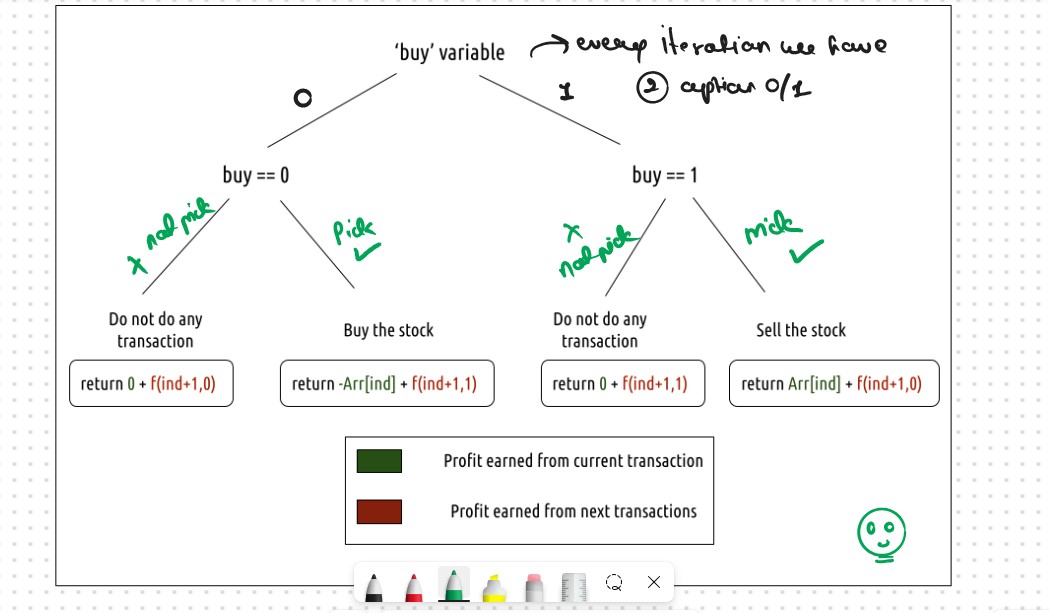
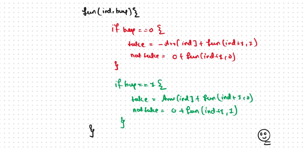
Every day, we have two choices

To either buy/sell the stock(based on the buy variable’s value and if ‘cap’ > 0).

To do nothing and move on to the next day.

If We Carefully Observed then we see this Probelem Base on the pick/notPick concept that we do in the our Entire dp Playlist.

Case 1: When buy == 0, we can buy the stock.

If we can buy the stock on a particular day, we have two options

Option 1: To do no transaction and move to the next day. In this case, the net profit earned will be 0 from the current transaction, and to calculate the maximum profit starting from the next day, we will recursively call f(ind+1,0). As we have not bought the stock, the ‘buy’ variable value will still remain 0, indicating that we can buy the stock the next day. And the ‘cap’ variable will remain the same as if no transaction took place. (notTake)

Option 2: The other option is to buy the stock on the current day. In this case, the net profit earned from the current transaction will be -Arr[i]. As we are buying the stock, we are giving money out of our pocket, therefore the profit we earn is negative. To calculate the maximum profit starting from the next day, we will recursively call f(ind+1,1). As we have bought the stock, the ‘buy’ variable value will change to 1, indicating that we can’t buy and only sell the stock the next day. As we have only bought the stock and not sold it the transaction remains incomplete and the ‘cap’ variable value remains unchanged.(Take)

Case 2: When buy == 1, we can sell the stock.

Agin we have If we can buy the stock on a particular day, we have two options

Option 1: To do no transaction and move to the next day. In this case, the net profit earned will be 0 from the current transaction, and to calculate the maximum profit starting from the next day, we will recursively call f(ind+1,1). As we have not bought the stock, the ‘buy’ variable value will still remain at 1, indicating that we can’t buy and only sell the stock the next day. And the ‘cap’ variable will remain the same as if no transaction took place.notTake

Option 2: The other option is to sell the stock on the current day. In this case, the net profit earned from the current transaction will be +Arr[i]. As we are selling the stock, we are putting the money into our pocket, therefore the profit we earn is positive. To calculate the maximum profit starting from the next day, we will recursively call f(ind+1,0). As we have sold the stock, the ‘buy’ variable value will change to 0, indicating that we can buy the stock the next day. As we have sold the earlier bought stock, we make one complete transaction, therefore now we update the ‘cap’ variable’s value to cap-1.Take

The figure below gives us the Summary

Step 3: Return the Maximum

As we are looking to maximize the profit earned, we will return the maximum value in both cases. The final pseudocode after steps 1, 2, and 3

Base Cases

If ind==n, it means we have finished trading on all days, and there is no more money that we can get, therefore we simply return 0. ("Does.t Matter if we Have Some Stocks are Remaing not at the End Profit will we 0")

If cap==0, it means that we cannot make any more transactions. Therefore we return 0.

Recursion Python Code

class Solution:
        
    def RecursionApproch(self, prices,index,n,decisionFlag,transactionLimit):
        
        # Base Case    
        if index == n or transactionLimit == 0:
            return 0
                
        maxProfit = 0
                
        if decisionFlag == 1:
            # as similar to take and notTake Concepts
            buyTheStock = -prices[index] + self.RecursionApproch(prices,index+1,n,0,transactionLimit)
            notBuyTheStock = 0 + self.RecursionApproch(prices,index+1,n,1,transactionLimit)
            maxProfit = max(buyTheStock,notBuyTheStock)
           
        else:
            shellTheStock = prices[index] + self.RecursionApproch(prices, index + 1, n, 1,transactionLimit-1)
            notSellTheStock = 0 + self.RecursionApproch(prices, index + 1, n, 0,transactionLimit)
            maxProfit = max(shellTheStock, notSellTheStock)
                    
        return maxProfit

    def maxProfit(self, prices):
                 
        n = len(prices)
        decisionFlag = 1
        transactionLimit = 2
        
        return self.RecursionApproch(prices,0,n,decisionFlag,transactionLimit)

ans = Solution()
prices = [3,3,5,0,0,3,1,4]
print(ans.maxProfit(prices))

Time & Space Complexity

Time Complexity: O(2^N)
Reason: Exponential Time we find out the all the Possible Path
Space Complexity: O(N)
Reason: We are using a recursion stack space(O(N))

Memoization Approch

If we Observe in the recursion tree, we will observe a many number of overlapping subproblems. Therefore the recursive solution can be memoized for to reduce the time complexity.

Steps to convert Recursive code to memoization solution:

The Twist in the Memoization we Used a 3D DP fro thsi Probelem where dp[n][2][3]
Where:-
n:- Size of the Input Array
2:- Dession Flag
3:- Cap Flag or Transaction Limit

Create a dp array of size [n][2][3]. The size of the input array is ‘n’, so the index will always lie between ‘0’ and ‘n-1’. The ‘buy’ variable can take only two values: 0 and 1 and the ‘cap’ variable can only take three variables 0, 1, and 2. Therefore we take the dp array as dp[n][2][3].

We initialize the dp array to -1.

Whenever we want to find the answer of particular parameters (say f(ind,buy,cap)), we first check whether the answer is already calculated using the dp array(i.e dp[ind][buy][cap]!= -1 ). If yes, simply return the value from the dp array.

If not, then we are finding the answer for the given value for the first time, we will use the recursive relation as usual but before returning from the function, we will set dp[ind][buy][cap] to the solution we get.

Memoization Python Code

class Solution:
        
    def MemoizationApproch(self, prices,index,n,decisionFlag,dp,transactionLimit):

        # Base Case
        if index == n or transactionLimit == 0:
            return 0
                
        if dp[index][decisionFlag][transactionLimit] != -1:
            return dp[index][decisionFlag][transactionLimit]

        maxProfit = 0
                
        if decisionFlag == 1:
            # as similar to take and notTake Concepts
            buyTheStock = -prices[index] + self.MemoizationApproch(prices,index+1,n,0,dp,transactionLimit)
            notBuyTheStock = 0 + self.MemoizationApproch(prices,index+1,n,1,dp,transactionLimit)
            maxProfit = max(buyTheStock,notBuyTheStock)
           
        else:
            shellTheStock = prices[index] + self.MemoizationApproch(prices, index + 1, n, 1,dp,transactionLimit-1)
            notSellTheStock = 0 + self.MemoizationApproch(prices, index + 1, n, 0,dp,transactionLimit)
            maxProfit = max(shellTheStock, notSellTheStock)
                    
        dp[index][decisionFlag][transactionLimit] = maxProfit
        # we can also return maxProfit its also give the correct answer
        return dp[index][decisionFlag][transactionLimit]

    def maxProfit(self, prices):
                 
        n = len(prices)
        decisionFlag = 1
        transactionLimit = 2
        
        dp = [[[-1 for _ in range(transactionLimit+1)] for _ in range(2)] for _ in range(n)]
   
        return self.MemoizationApproch(prices,0,n,decisionFlag,dp,transactionLimit)

ans = Solution()
prices = [3,3,5,0,0,3,1,4]
print(ans.maxProfit(prices))

Time & Space Complexity

Time Complexity:O(N*2*3)
Reason: There are N*2*3 states therefore at max ‘N*2*3’ new problems will be solved
Space Complexity: O(N*2*3) + O(N)
Reason: We are using a recursion stack space(O(N)) and a 3D array ( O(N*2*3)).

Tabulation Approch

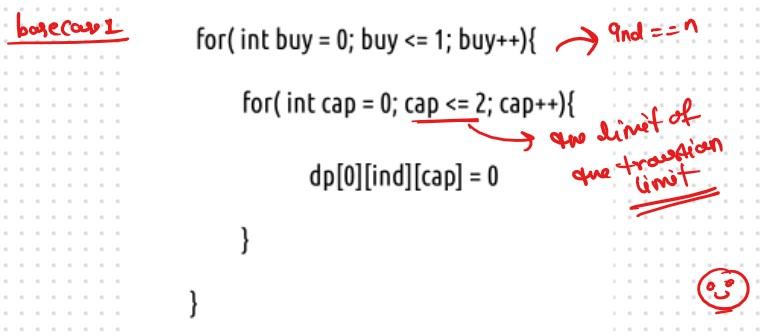
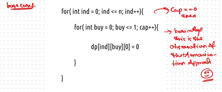
Tabulation is a ‘bottom-up’ approach where we start from the base case and reach the final answer that we want and Memoization is the Top-down Approch.

In Tabulation Approch We Just Creat a DP Array Same as Memoization and Simply Convert the Recurance Relation into the form of the Looping

VVVV Important Point: Tabulation Approch is Always 1-Based Indexing Always Remember

Steps to convert Recursive Solution to Tabulation one.

To convert the memoization approach to a tabulation one, create a dp array with the same size as done in memoization. We can initialize it as 0. (size [N+1][2][3])

Handling the base Case Now, what the base condition in the recursive relation is

if( ind == n || cap == 0) return 0 We handle this in the following way

ind == n When ind == n, the other two variables: cap and buy can take any value, therefore we can set the following two loops and set dp[n][buy][cap] = 0

cap == 0 When cap == 0, the other two variables: ind and cap can take any value, therefore we can set the following two loops and set dp[ind][buy][0] = 0.

Another hack is to initialize the entire 3D DP Array as 0. In this case, we need not worry about explicitly setting the base cases.

First, we declare the dp array of size [n+1][2][3] as zero.

As we have initialized the array as 0, we have automatically set the base condition as explained above.

Now, traverse the array in the opposite direction of that of the memoization technique. We will start from ind = n-1 -> ind =0.

In every iteration copy the recursive code logic.

At last dp[0][0][2] ( maximum profit generated on ith day, when we can buy the stock on 0th day and can have a total 2 transactions) gives us the final answer.

VVVVVVV Imp Point

We All Ready Inilisezed the Our Entire DP array with 0, No Need to write the base case all ready all zero but we write the base case for the understanding the Tabulation Approch

Tabulation Python Code

class Solution:
        
    def TabulationApproch(self, prices,n,dp):
        
        # Base Case
        # if index == n
        
        for index in range(2):
            for currdecisionFlag in range(3):
                dp[0][index][currdecisionFlag] = 0


        # if transactionLimit == 0
        for index in range(n):
            for currdecisionFlag in range(2):
                dp[index][currdecisionFlag][0] = 0

        print(dp)

        # Important Note: We All Ready in our DP inilisezed with the 0, no need to write the Base
        # Case allready all 0, But we Write the Base Case for the Understanding the Tabulation

        for index in range(n-1,-1,-1):
            for decisionFlag in range(2):
                for transactionLimit in range(1,3):

                    maxProfit = 0
                    if decisionFlag == 1:
                        # as similar to take and notTake Concepts
                        buyTheStock = -prices[index] + dp[index + 1][0][transactionLimit]
                        notBuyTheStock = 0 + dp[index + 1][1][transactionLimit]
                        maxProfit = max(buyTheStock,notBuyTheStock)
                    

                    else:
                        shellTheStock = prices[index] + dp[index + 1][1][transactionLimit-1]
                        notSellTheStock = 0 + dp[index + 1][0][transactionLimit]
                        maxProfit = max(shellTheStock, notSellTheStock)
                    

                    dp[index][decisionFlag][transactionLimit] = maxProfit

        # we can also return maxProfit its also give the correct answer
        print(dp)
        return dp[0][1][2]

    def maxProfit(self, prices):
                 
        n = len(prices)
        transactionLimit = 2
        dp = [[[0 for _ in range(transactionLimit+1)] for _ in range(2)] for _ in range(n+1)]
        
        print(dp)
        return self.TabulationApproch(prices,n,dp)

ans = Solution()
prices = [3,3,5,0,0,3,1,4]
print(ans.maxProfit(prices))

Time & Space Complexity

Time Complexity: O(N*2*3)
Reason: There are three nested loops that account for O(N*2*3) complexity.
Space Complexity: O(N*2*3)
Reason: We are using an external array of size ‘N*2*3’. Stack Space is eliminated.

Space Optimization

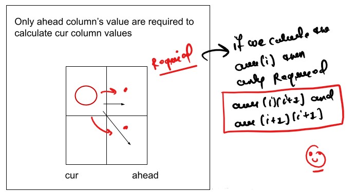
If we closelly Observed if any Tabulation Approch we used the Some Limited Stuff like: dp[ind][buy][cap] = max(dp[ind+1][buy][cap] , max( dp[ind+1][!buy][cap])) for the finding the our ans then definetly here Spaced Optimization is Possible in that types of Problems. Always Remember

Golden Rule

If we required only Prev row and Prev Collom then definetly we can Space Optimized

We see that to calculate a value of a cell of the dp array, we need only the next column values(say ahead). So, we don’t need to store an entire 2-D array. Hence we can space optimize it.

We take two rows ‘prev’ and ‘cur’

We set a 2D vector ahead initialized to 0 (base condition) and another 2D

Then we set three nested loops to calculate the cur array’s values.

We replace dp[ind] with cur and dp[ind+1] with ahead in our tabulation code.

After the inner loop execution, we set ahead as cur for the next outer loop iteration.

At last, we return prev[1][2] as our answer.

Some Important Points:

prev = curr: Some Time not working and not give a Correct answer, same like we face in this Problem due to the Dynamic element Allocation

So we try at the place of the prev = curr

prev[:] = curr

prev = curr[:]

SpaceOptmized Python Code

class Solution:
        
    def SpaceOptimizationApproch(self, prices,n,prev,curr):

        # Base Case
        # if index == n
        
        for index in range(2):
            for currdecisionFlag in range(3):
                prev[0][currdecisionFlag] = 0


        # if transactionLimit == 0
        for index in range(n):
            for currdecisionFlag in range(2):
                prev[currdecisionFlag][0] = 0

        print(prev)
        print(curr)

        # Important Note: We All Ready in our DP inilisezed with the 0, no need to write the Base
        # Case allready all 0, But we Write the Base Case for the Understanding the Tabulation

        for indx in range(n-1,-1,-1):
            for decisionFlag in range(2):
                for transactionLimit in range(1,3):

                    maxProfit = 0
                    if decisionFlag == 1:
                        # as similar to take and notTake Concepts
                        buyTheStock = -prices[indx] + prev[0][transactionLimit]
                        notBuyTheStock = 0 + prev[1][transactionLimit]
                        maxProfit = max(buyTheStock,notBuyTheStock)
                        

                    else:
                        shellTheStock = prices[indx] + prev[1][transactionLimit-1]
                        notSellTheStock = 0 + prev[0][transactionLimit]
                        maxProfit = max(shellTheStock, notSellTheStock)
                        

                    curr[decisionFlag][transactionLimit] = maxProfit
                
                prev = curr

        # we can also return maxProfit its also give the correct answer
        return prev[1][2]

    def maxProfit(self, prices):
                 
        n = len(prices)

        prev = [[0  for _ in range(3)]  for _ in range(2)]
        curr = [[0  for _ in range(3)]  for _ in range(2)]

        return self.SpaceOptimizationApproch(prices,n,prev,curr)

ans = Solution()
prices = [3,3,5,0,0,3,1,4]
print(ans.maxProfit(prices))

Time & Space Complexity

Time Complexity: O(N*2)
Reason: There are two nested loops that account for O(N*2) complexity
Space Complexity: O(1)
Reason: We are using an external array of size ‘2’.

Most Space Optimization

If we observe very carefully, then its Possible to Optimized our Space frpm 3D DP to (N*4) DP Memoization, Tabulation and Space Optimized Possible ley's Understand How ?

What is N * 4 DP Solution
In our Solution what we do fun(cap,transcationLimit) if transcationLimit == 0 then we formed our Solution that we Discuss

So This Approch is the Completely Observation Based Approch
We know that we have the 2 transcationLimit that means 4 Options

    Buy  Shell  Buy  Shell
     0     1     2     3

So here we Observed very Carefully our buy transcation will only then index % 2 == 0 (even) otherwise shell

That is the Core Concept that we used to Convert the our 3D DP Solution into the 2D DP Solution in All the Formate Memoization, Tabulation and Space Optimized

Recursion Optmized Python Code

class Solution:
        
    def RecursionApproch(self, prices,index,n,transactionLimit):
        
        # Base Case    
        if index == n or transactionLimit == 4:
            return 0
                
        maxProfit = 0
                
        if transactionLimit % 2 == 0:
            # as similar to take and notTake Concepts
            buyTheStock = -prices[index] + self.RecursionApproch(prices,index+1,n,transactionLimit+1)
            notBuyTheStock = 0 + self.RecursionApproch(prices,index+1,n,transactionLimit)
            maxProfit = max(buyTheStock,notBuyTheStock)
           
        else:
            shellTheStock = prices[index] + self.RecursionApproch(prices, index + 1, n ,transactionLimit+1)
            notSellTheStock = 0 + self.RecursionApproch(prices, index + 1, n ,transactionLimit)
            maxProfit = max(shellTheStock, notSellTheStock)
                    
        return maxProfit

    def maxProfit(self, prices):
                 
        n = len(prices)
        transactionLimit = 0
        return self.RecursionApproch(prices,0,n,transactionLimit)

ans = Solution()
prices = [3,3,5,0,0,3,1,4]
print(ans.maxProfit(prices))

Memoization Optmized Python Code

class Solution:
        
    def MemoizationApproch(self, prices, index, n, dp, transactionLimit):

        # Base Case
        if index == n or transactionLimit == 4:
            return 0
                
        if dp[index][transactionLimit] != -1:
            return dp[index][transactionLimit]

        maxProfit = 0
                
        if transactionLimit % 2 == 0:
            # as similar to take and notTake Concepts
            buyTheStock = -prices[index] + self.MemoizationApproch(prices,index+1,n,dp,transactionLimit+1)
            notBuyTheStock = 0 + self.MemoizationApproch(prices,index+1,n,dp,transactionLimit)
            maxProfit = max(buyTheStock,notBuyTheStock)
           
        else:
            shellTheStock = prices[index] + self.MemoizationApproch(prices, index + 1, n ,dp,transactionLimit+1)
            notSellTheStock = 0 + self.MemoizationApproch(prices, index + 1, n ,dp,transactionLimit)
            maxProfit = max(shellTheStock, notSellTheStock)
                    
        dp[index][transactionLimit] = maxProfit
        # we can also return maxProfit its also give the correct answer
        return dp[index][transactionLimit]

    def maxProfit(self, prices):
                 
        n = len(prices)
        transactionLimit = 0

        dp = [[-1 for _ in range(4)] for _ in range(n)]
   
        return self.MemoizationApproch(prices, 0, n, dp, transactionLimit)

ans = Solution()
prices = [3,3,5,0,0,3,1,4]
print(ans.maxProfit(prices))

Tabulation Optmized Python Code

class Solution:
        
    def TabulationApproch(self, prices,n,dp):
        
        # Base Case
        # if index == n
        
        for index in range(5):
            dp[n][index] = 0


        # if transactionLimit == 0
        for index in range(n+1):
            dp[index][4]= 0

        print(dp)

        # Important Note: We All Ready in our DP inilisezed with the 0, no need to write the Base
        # Case allready all 0, But we Write the Base Case for the Understanding the Tabulation

        for index in range(n-1,-1,-1):
            for transactionLimit in range(3,-1,-1):
                
                maxProfit = 0
                if transactionLimit % 2 == 0:
                    # as similar to take and notTake Concepts
                    buyTheStock = -prices[index] + dp[index + 1][transactionLimit+1]
                    notBuyTheStock = 0 + dp[index + 1][transactionLimit]
                    maxProfit = max(buyTheStock,notBuyTheStock)
                

                else:
                    shellTheStock = prices[index] + dp[index + 1][transactionLimit+1]
                    notSellTheStock = 0 + dp[index + 1][transactionLimit]
                    maxProfit = max(shellTheStock, notSellTheStock)
                

                dp[index][transactionLimit] = maxProfit

        # we can also return maxProfit its also give the correct answer
        print(dp)
        return dp[0][0]

    def maxProfit(self, prices):
                 
        n = len(prices)
        transactionLimit = 0

        dp = [[0 for _ in range(5)] for _ in range(n+1)]
        
        print(dp)
        return self.TabulationApproch(prices,n,dp)

ans = Solution()
prices = [3,3,5,0,0,3,1,4]
print(ans.maxProfit(prices))

SpaceOptimized Optmized Python Code

class Solution:
        
    def SpaceOptimizationApproch(self, prices,n,prev,curr):

        # Base Case
        # if index == n
        
        for index in range(5):
            prev[index] = 0

        # if transactionLimit == 0
        curr[4] = 0

        print(prev)
        print(curr)

        # Important Note: We All Ready in our DP inilisezed with the 0, no need to write the Base
        # Case allready all 0, But we Write the Base Case for the Understanding the Tabulation

        for indx in range(n-1,-1,-1):
            for transactionLimit in range(3,-1,-1):
                
                maxProfit = 0
                if transactionLimit % 2 == 0:
                    # as similar to take and notTake Concepts
                    buyTheStock = -prices[indx] + prev[transactionLimit+1]
                    notBuyTheStock = 0 + prev[transactionLimit]
                    maxProfit = max(buyTheStock,notBuyTheStock)
                    

                else:
                    shellTheStock = prices[indx] + prev[transactionLimit+1]
                    notSellTheStock = 0 + prev[transactionLimit]
                    maxProfit = max(shellTheStock, notSellTheStock)
                    
                curr[transactionLimit] = maxProfit
                
            prev = curr

        # we can also return maxProfit its also give the correct answer
        return prev[0]

    def maxProfit(self, prices):
                 
        n = len(prices)
        transactionLimit = 0
        prev = [0]*5
        curr = [0]*5
        

        return self.SpaceOptimizationApproch(prices,n,prev,curr)

ans = Solution()
prices = [3,3,5,0,0,3,1,4]
print(ans.maxProfit(prices))

Time & Space Complexity

Time Complexity: O(N*2)
Reason: There are two nested loops that account for O(N*2) complexity
Space Complexity: O(5)
Reason: We are using just Size of 5(len) DP 1D Array prev and curr.

Most Space Optimization Using 4 Variables

This Approch is a popular approach on platforms like LeetCode however, it often lacks a clear intuition behind the logic. Recruiters may not be satisfied with solutions that utilize four variables without a valid and authenticated rationale. Therefore, it is advisable not to present this approach in interviews. Nevertheless, I have included this solution for the purpose of understanding and learning.

SpaceOptmized Python Code

class Solution:
        
    def MostSpaceOptimizationApproch(self, prices, n):

        if not prices:
            return 0
        
        A = -prices[0]
        B = float('-inf')
        C = float('-inf')
        D = float('-inf')

        for price in prices:
            A = max(A, -price)
            B = max(B, A + price)
            C = max(C, B - price)
            D = max(D, C + price)
            
        return D

    def maxProfit(self, prices):
                 
        n = len(prices)
        return self.MostSpaceOptimizationApproch(prices, n)

ans = Solution()
prices = [3,3,5,0,0,3,1,4]
print(ans.maxProfit(prices))

Time & Space Complexity

Time Complexity: O(N)
Reason: There are two nested loops that account for O(N*2) complexity
Space Complexity: O(4)
Reason: We are using just used 4 Variable.

Color

Background

Interview Docs File "All the Best" Team @DSAwithPrinceSingh

~ It's All About Consistency📈 Dedication🎯 HardWork💪 Happy Coding❤️ ~