Jb Tak Fodega Nhi 🎯 Tb Tk Chodega Nhi 📚 (MAANG)

DP39 Buy and Sell Stocks With Cooldown

We are given an array Arr[] of length n. It represents the price of a stock on ‘n’ days. The following guidelines need to be followed:

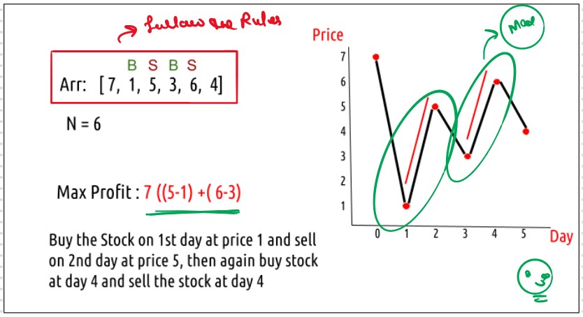
We can buy and sell the stock any number of times.

In order to sell the stock, we need to first buy it on the same or any previous day.

We can’t buy a stock again after buying it once. In other words, we first buy a stock and then sell it. After selling we can buy and sell again. But we can’t sell before buying and can’t buy before selling any previously bought stock.

We can’t buy a stock on the very next day of selling it. This is the cooldown clause.

Find and return the maximum profit you can achieve.

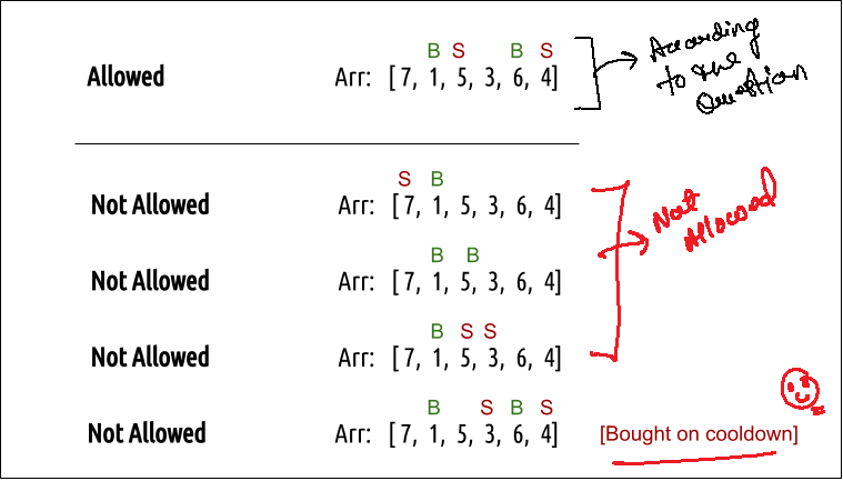
Every day, we will have two choices, either to do nothing and move to the next day or to buy/sell (based on the last transaction) and find out the profit. Therefore we need to generate all the choices in order to compare the profit. As we need to try out all the possible choices, we will use recursion.

In Best Time to Buy and Sell Stock I: We Allow Just Only 1 Transactions

In Best Time to Buy and Sell Stock II: We Allow Infinite Transactions

In Best Time to Buy and Sell Stock III: We Allow Just Only 2 Transactions

In Best Time to Buy and Sell Stock IV: We Allow Just K Transactions

In Best Time to Buy and Sell Stock V: We Allow Infinite Transactions with Cooldown

How Can I Solved this Problme and How I Link this Problem to the DP on Stock II

Generally We Follow the Same Approch and Logic that we follow in the DP on Stock II but here is the Slight Modification that is Cooldown

this is the Recursive Solution of the DP on Stock II with Slight Modification
What is teh Change and the Change is Only When we shellTheStock then Just the place of index+1 we did it index+2 this is the Only change and Entire Remaining Code and Concept wii be Same as We do in the DP on Stock II

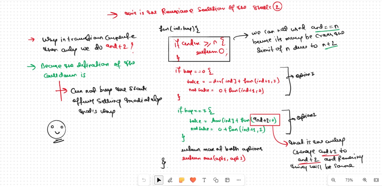
Now the Question is Why ? we do index+2 at the Time of shellTheStock Only

Becouse the Defination of the Cooldown is We Can Not Buy the Stock after Shelling the Stock Imedietely that's why

We increment the Index+2 atthe Time of Transactions Completion

Now Remaining Entire 👇 Process will Be Same As Like in DPL36

Recursice Approch

Again here we follow the out Standerad Patter that we learned in the Dynamic Programming Introduction. How to Write Recursion

Steps to form the Recursive Solution
Step 1: Express the problem in terms of indexes.

We need to think in the terms of the number of days, therefore one variable will be the array index( say ind). Next, we need to respect the condition that we can’t buy a stock again, that is we need to first sell a stock, and then we can buy that again. Therefore we need a second variable ‘buy’ which tells us on a particular day whether we can buy or sell the stock.

Step 2: Try out all possible choices at a given index.

Every day, we have two choices

To either buy/sell the stock(based on the buy variable’s value).

To do nothing and move on to the next day.

If We Carefully Observed then we see this Probelem Base on the pick/notPick concept that we do in the our Entire dp Playlist.

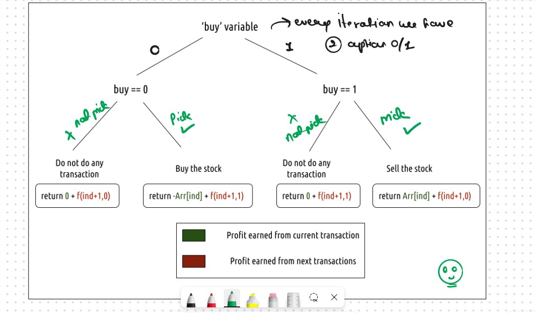
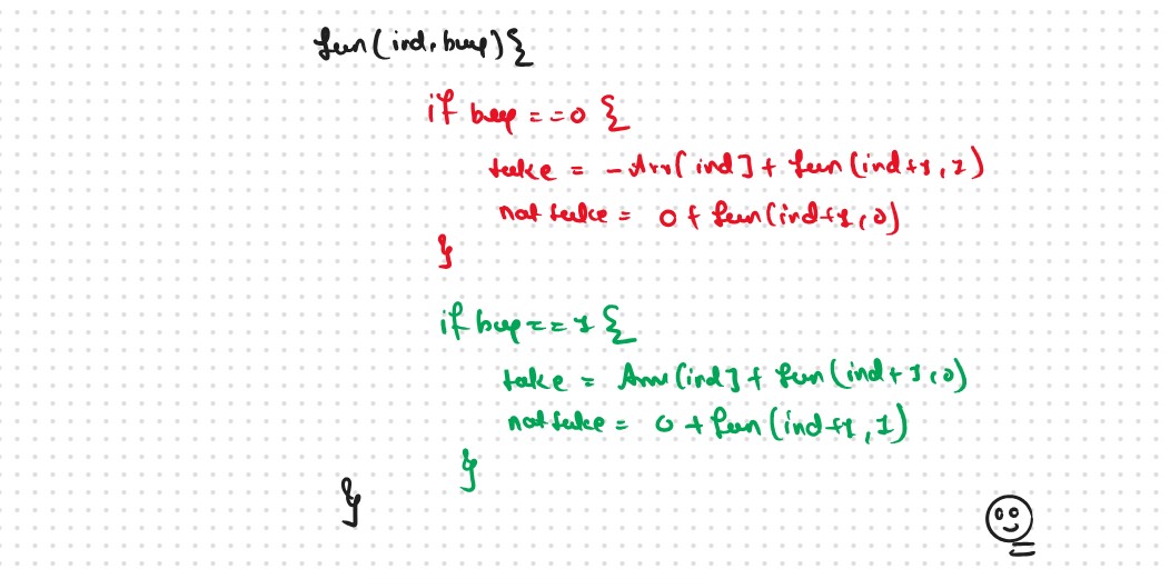
Case 1: When buy == 0, we can buy the stock.

If we can buy the stock on a particular day, we have two options

Option 1: To do no transaction and move to the next day. In this case, the net profit earned will be 0 from the current transaction, and to calculate the maximum profit starting from the next day, we will recursively call f(ind+1,0). As we have not bought the stock, the ‘buy’ variable value will still remain 0, indicating that we can buy the stock the next day. (notTake)

Option 2: The other option is to buy the stock on the current day. In this case, the net profit earned from the current transaction will be -Arr[i]. As we are buying the stock, we are giving money out of our pocket, therefore the profit we earn is negative. To calculate the maximum profit starting from the next day, we will recursively call f(ind+1,1). As we have bought the stock, the ‘buy’ variable value will change to 1, indicating that we can’t buy and only sell the stock the next day. (Take)

Case 2: When buy == 1, we can sell the stock.

Agin we have If we can buy the stock on a particular day, we have two options

Option 1: To do no transaction and move to the next day. In this case, the net profit earned will be 0 from the current transaction, and to calculate the maximum profit starting from the next day, we will recursively call f(ind+1,1). As we have not bought the stock, the ‘buy’ variable value will still remain at 1, indicating that we can’t buy and only sell the stock the next day. notTake

Option 2: The other option is to sell the stock on the current day. In this case, the net profit earned from the current transaction will be +Arr[i]. As we are selling the stock, we are putting the money into our pocket, therefore the profit we earn is positive. To calculate the maximum profit starting from the next day, we will recursively call f(ind+1,0). As we have sold the stock, the ‘buy’ variable value will change to 0, indicating that we can buy the stock the next day. Take

The figure below gives us the Summary

Step 3: Return the Maximum

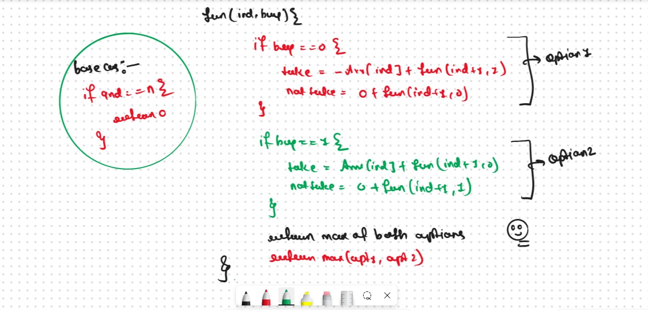
As we are looking to maximize the profit earned, we will return the maximum value in both cases. The final pseudocode after steps 1, 2, and 3

Base Cases If ind>=n, (Index+2 May Be Excied the Limit of the Index) it means we have finished trading on all days, and there is no more money that we can get, therefore we simply return 0. ("Does.t Matter if we Have Some Stocks are Remaing not at the End Profit will we 0")

Recursion Python Code

class Solution:
        
    def RecursionApproch(self, prices,index,n,decisionFlag):
        
        # Base Case >= Becouse Index+2 May Be Excied the Limit of the Index    
        if index >= n:
            return 0
                
        maxProfit = 0
                
        if decisionFlag == 1:
            # as similar to take and notTake Concepts
            buyTheStock = -prices[index] + self.RecursionApproch(prices,index+1,n,0)
            notBuyTheStock = 0 + self.RecursionApproch(prices,index+1,n,1)
            maxProfit = max(buyTheStock,notBuyTheStock)
           
        else:
            shellTheStock = prices[index] + self.RecursionApproch(prices, index + 2, n, 1)
            notSellTheStock = 0 + self.RecursionApproch(prices, index + 1, n, 0)
            maxProfit = max(shellTheStock, notSellTheStock)
                    
        return maxProfit

    def maxProfit(self, prices):
                 
        n = len(prices)
        decisionFlag = 1
        return self.RecursionApproch(prices,0,n,decisionFlag)

ans = Solution()
prices = [1,2,3,0,2]
print(ans.maxProfit(prices))

Time & Space Complexity

Time Complexity: O(2^N)
Reason: Exponential Time we find out the all the Possible Path
Space Complexity: O(N)
Reason: We are using a recursion stack space(O(N))

Memoization Approch

If we Observe in the recursion tree, we will observe a many number of overlapping subproblems. Therefore the recursive solution can be memoized for to reduce the time complexity.

Steps to convert Recursive code to memoization solution:

Create a dp array of size [n][2]. The size of the input array is ‘n’, so the index will always lie between ‘0’ and ‘n-1’. The ‘buy’ variable can take only two values: 0 and 1. Therefore we take the dp array as dp[n][2]

We initialize the dp array to -1.

Whenever we want to find the answer to particular parameters (say f(ind, buy)), we first check whether the answer is already calculated using the dp array(i.e dp[ind][buy]!= -1 ). If yes, simply return the value from the dp array.

If not, then we are finding the answer for the given value for the first time, we will use the recursive relation as usual but before returning from the function, we will set dp[ind][buy] to the solution we get.

Memoization Python Code

class Solution:
        
    def MemoizationApproch(self, prices,index,n,decisionFlag,dp):

        # Base Case
        if index >= n:
            return 0
                
        if dp[index][decisionFlag] != -1:
            return dp[index][decisionFlag]

        maxProfit = 0
                
        if decisionFlag == 1:
            # as similar to take and notTake Concepts
            buyTheStock = -prices[index] + self.MemoizationApproch(prices,index+1,n,0,dp)
            notBuyTheStock = 0 + self.MemoizationApproch(prices,index+1,n,1,dp)
            maxProfit = max(buyTheStock,notBuyTheStock)
           
        else:
            shellTheStock = prices[index] + self.MemoizationApproch(prices, index + 2, n, 1,dp)
            notSellTheStock = 0 + self.MemoizationApproch(prices, index + 1, n, 0,dp)
            maxProfit = max(shellTheStock, notSellTheStock)
                    
        dp[index][decisionFlag] = maxProfit
        # we can also return maxProfit its also give the correct answer
        return dp[index][decisionFlag]

    def maxProfit(self, prices):
                 
        n = len(prices)
        decisionFlag = 1
        dp = []
        for _ in range(n):
            arr = [-1] * (2)
            dp.append(arr)
        return self.MemoizationApproch(prices,0,n,decisionFlag,dp)

ans = Solution()
prices = [1,2,3,0,2]
print(ans.maxProfit(prices))

Time & Space Complexity

Time Complexity:O(N*2)
Reason: TThere are N*2 states therefore at max ‘N*2’ new problems will be solved and we are running a for loop for ‘N’ times to calculate the total sum
Space Complexity: O(N*2) + O(N)
Reason: We are using a recursion stack space(O(N)) and a 2D array ( O(N*2)).

Tabulation Approch

Tabulation is a ‘bottom-up’ approach where we start from the base case and reach the final answer that we want and Memoization is the Top-down Approch.

In Tabulation Approch We Just Creat a DP Array Same as Memoization and Simply Convert the Recurance Relation into the form of the Looping

VVVV Important Point: Tabulation Approch is Always 1-Based Indexing Always Remember

Steps to convert Recursive Solution to Tabulation one.

To convert the memoization approach to a tabulation one, create a dp array with the same size as done in memoization. We can initialize it as 0. (size [n+1][2] as zero)

Next, we set two nested for loops, the outer loop (for variable ind) moves from n-1 to 0 and the inner loop (for variable buy) moves from 0 to 1.

In every iteration, we calculate the value according to the memoization logic.

At last, we will print dp[0][1] as our answer.

Tabulation Python Code

class Solution:
        
    def TabulationApproch(self, prices,n,dp):

        # Base Case
        dp[n][0] = 0
        dp[n][1] = 0

        for index in range(n-1,-1,-1):
            for decisionFlag in range(2):

                maxProfit = 0
                if decisionFlag == 1:
                    # as similar to take and notTake Concepts
                    buyTheStock = -prices[index] + dp[index+1][0]
                    notBuyTheStock = 0 + dp[index+1][1]
                    maxProfit = max(buyTheStock,notBuyTheStock)
                

                else:
                    shellTheStock = prices[index] + dp[index+2][1]
                    notSellTheStock = 0 + dp[index+1][0]
                    maxProfit = max(shellTheStock, notSellTheStock)
                

                dp[index][decisionFlag] = maxProfit

        # we can also return maxProfit its also give the correct answer
        print(dp)
        return dp[0][1]

    def maxProfit(self, prices):
                 
        n = len(prices)
        decisionFlag = 1
        dp = []
        for _ in range(n+2):
            arr = [0] * (2)
            dp.append(arr)
        print(dp)
        return self.TabulationApproch(prices,n,dp)

ans = Solution()
prices = [1,2,3,0,2]
print(ans.maxProfit(prices))

Time & Space Complexity

Time Complexity: O(N*2)
Reason: There are two nested loops that account for O(N*2) complexity.
Space Complexity: O(N*2)
Reason: We are using an external array of size ‘N*2’. Stack Space is eliminated.

Space Optimization

Ideally Space Optimization Not be Considered Becouse we have 3 Different - Different Parameter that is

Index+1

Index+2

Curr Index

3 Different Array Required that means its not worth it and its Occupied the Space like in Tabulation that's Why Not Space Optimization Not Required in this Question

But We Do Space Optimization also for the Better Understandbality

If we closelly Observed if any Tabulation Approch we used the Some Limited Stuff like: dp[ind][buy] = max(dp[ind+1][buy] , max( dp[ind+1][!buy])) for the finding the our ans then definetly here Spaced Optimization is Possible in that types of Problems. Always Remember

Golden Rule

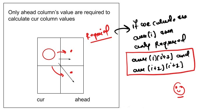
If we required only Prev row and Prev Collom then definetly we can Space Optimized

We see that to calculate a value of a cell of the dp array, we need only the next column values(say ahead). So, we don’t need to store an entire 2-D array. Hence we can space optimize it.

We take two rows ‘prev’ and ‘cur’

Then we set the nested loops to calculate the cur column values.

We replace dp[ind] with cur and dp[ind+1] with prev in our memoization code.

Next, we implement the memoization logic. We replace dp[i-1] with prev and dp[i] by cur

After the inner loop execution, we set ahead as cur for the next outer loop iteration.

At last, we return prev[1] as our answer.

Some Important Points:

prev = curr: Some Time not working and not give a Correct answer, same like we face in this Problem due to the Dynamic element Allocation

So we try at the place of the prev = curr

prev[:] = curr

prev = curr[:]

SpaceOptmized Python Code

class Solution:
        
    def SpaceOptimizationApproch(self, prices,n,curr,prev1,prev2):
        
        # Important Note: We All Ready in our DP inilisezed with the 0, no need to write the Base
        # Case allready all 0, But we Write the Base Case for the Understanding the Tabulation
        
        for index in range(n-1,-1,-1):
            for decisionFlag in range(2):

                maxProfit = 0
                if decisionFlag == 0:
                    # as similar to take and notTake Concepts
                    buyTheStock = -prices[index] + prev1[1]
                    notBuyTheStock = 0 + prev1[0]
                    maxProfit = max(buyTheStock,notBuyTheStock)
                

                else:
                    shellTheStock = prices[index] + prev2[0]
                    notSellTheStock = 0 + prev1[1]
                    maxProfit = max(shellTheStock, notSellTheStock)
                

                curr[decisionFlag] = maxProfit
            
            
            prev2 = prev1.copy()
            prev1 = curr.copy()
            

        # we can also return maxProfit its also give the correct answer
        return curr[0]

    def maxProfit(self, prices):
                 
        n = len(prices)
        curr = [0,0]
        prev1 = [0,0]
        prev2 = [0,0]
        return self.SpaceOptimizationApproch(prices,n,curr,prev1,prev2)

ans = Solution()
prices = [1,2,3,0,2]
print(ans.maxProfit(prices))

Time & Space Complexity

Time Complexity: O(N*2)
Reason: There are two nested loops that account for O(N*2) complexity
Space Complexity: O(1)
Reason: We are using an external array of size ‘2’.

Most Space Optimization

Ideally Space Optimization Not be Considered Becouse we have 3 Different - Different Parameter that is

Index+1

Index+2

Curr Index

3 Different Array Required that means its not worth it and its Occupied the Space like in Tabulation that's Why Not Space Optimization Not Required in this Question

But We definetly bypass the Ineer loop of the Tabulation Approch that we do in the Tabulation Approch

I Know that if index == 1 then buy and index == 0 then sell

Used this Concept for the By Pass the Inner Loop

If we observe very carefully, we only require two variables, namely prices[index + 1] and prices[index], for calculating the current day's profit. That's it; this is the crux of the question. We just use these two entities, and with each iteration, we update the profit.

Most SpaceOptmized Python Code

class Solution:
        
    def TabulationApproch(self, prices,n,dp):
            
        # Base Case
        dp[n][0] = 0
        dp[n][1] = 0

        for index in range(n-1,-1,-1):
                                                  
            maxProfit = 0

            # as similar to take and notTake Concepts
            buyTheStock = -prices[index] + dp[index+1][0]
            notBuyTheStock = 0 + dp[index+1][1]
            maxProfit = max(buyTheStock,notBuyTheStock)
            dp[index][1] = maxProfit

            shellTheStock = prices[index] + dp[index+2][1]
            notSellTheStock = 0 + dp[index+1][0]
            maxProfit = max(shellTheStock, notSellTheStock)
            dp[index][0] = maxProfit

        # we can also return maxProfit its also give the correct answer
        print(dp)
        return dp[0][1]

    def maxProfit(self, prices):
                 
        n = len(prices)
        dp = []
        for _ in range(n+2):
            arr = [0] * (2)
            dp.append(arr)
        
        print(dp)

        return self.TabulationApproch(prices,n,dp)

ans = Solution()
prices = prices = [1,2,3,0,2]
print(ans.maxProfit(prices))

Time & Space Complexity

Time Complexity: O(N)
Reason: Linear Iteration we used only
Space Complexity: O(1)
Reason: We are using just 2 variables of the calculating the Profte.

Color

Background

Interview Docs File "All the Best" Team @DSAwithPrinceSingh

~ It's All About Consistency📈 Dedication🎯 HardWork💪 Happy Coding❤️ ~